library(purrr)
library(tidyverse)
library(ggplot2)
library(knitr)
library(spatstat)
theme_set(theme_minimal())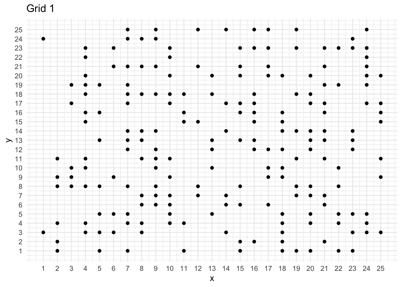
load packages
We have three grids available showing different patterns. How to test if the pattern is randomly distributed?
First I extracted all points with value of one and coded their coordinates: x-coordinate is the row number and y-coordinate is the column number. Then I got a list of points with their cooordinates. I converted this new data frame to a spatial ppp object. The problem becomes to test for complete spatial randomness (CSR). I chose to use K-function to test CSR. K function is defined as \(K(h) = \frac{1}{\lambda}E\) \(\lambda\) here represents the intensity of events within distance h. E here is the number of events. In order to estimate the k-function, we can construct a cricle of radius h around each point event(i), count the number of each events(j) that fall inside this circle and repeat these two steps for all points(i) and sum up results. \(\hat K(h) = \frac{R}{n^2}\sum\sum_{i\neq j}\frac{I_h(d_{ij})}{W_{ij}}\). Here R is the area, n is the number of points, \(I_h(d_{ij})\) equals 1 if \(d_{ij} \leq h\), and 0 otherwise, \(W_{ij}\) is the edge correction - the proportion of circumferences of circle = 1 if whole circle in the study area). Under the assumption of CSR, the expected number of events within distance h of an event is \(K(h) = \pi h^2\). \(K(h) < \pi h^2\) if point pattern is regular and \(K(h) > \pi h^2\) if point pattern is clustered. I used envelope function to help calculate the K(h) for observed grid. Also I did 99 simulation - created 99 random patterns, and caculated K(h) for each iteration. Monte Carlo method was used to compute confidence interval. Since there is 99 simiulation, the significance level is 1/(99 + 1) which is 0.01. If the observed K(h) is above the upper bound of the confidence interval, the grid is showing some clustered patterns. If the observed K(h) is within the confidence interval, the grid is showing random pattern. In order to perform 99 simulations, I created a function called random_pattern_generator. First, I randomly sampled 0 or 1 for each random point that I want. Then I converted this vector to a matrix. Points with value of 1 form the random pattern that I desire.
random_pattern_generator <- function(a){
temp_v <- sample(c(0, 1), a*a, replace = T)
temp_df <- data.frame(matrix(temp_v , a, a))
simdata <- data.frame(x = coordinate(temp_df)$x, y = coordinate(temp_df)$y) %>% filter(!is.na(x))
simdata_rr = ppp(simdata$x, simdata$y, window = owin(c(1,a),c(1,a)))
simdata_rr
}
Here, grid 1 and grid 2 are showing random patterns and grid 3 is showing clustering.
df <- read.table("./Grid1.txt", header = FALSE)

dim(df)
[1] 25 25# create a function to extract coordinates
coordinate <- function(database) {
# create blank vectors to store value
x <- rep(0, dim(database)[1] * dim(database)[2])
y <- rep(0, dim(database)[1] * dim(database)[2])
for (i in 1:dim(database)[1]) {
for (j in 1:dim(database)[2]) {
if (database[i, j] == 0) {
x[(i - 1) * dim(database)[2] + j] <- NA
y[(i - 1) * dim(database)[2] + j] <- NA
}
if (database[i, j] == 1) {
x[(i - 1) * dim(database)[2] + j] <- i
y[(i - 1) * dim(database)[2] + j] <- j
}
}
}
list(x = x, y = y)
}
mydata <- data.frame(x = coordinate(df)$x, y = coordinate(df)$y)
mydata <- mydata %>% filter(!is.na(x))
# visualize the grid
ggplot(mydata, aes(x = x, y = y)) +
geom_point() +
scale_x_continuous(breaks = seq(1, 25, 1)) +
scale_y_continuous(breaks = seq(1, 25, 1)) +
labs(title = "Grid 1")
# number of points

print(paste("Number of points: ", mydata %>% nrow()))
[1] "Number of points: 205"n <- mydata %>% nrow()
# create a spatial ppp object
mydata_rr <- ppp(mydata$x, mydata$y, window = owin(c(1, 25), c(1, 25)))
# Creating multiple random point patterns with n points and within the window
set.seed(2020)
# create a function to select n points randomly within the window
random_pattern_generator <- function(a) {
temp_v <- sample(c(0, 1), a * a, replace = T)
temp_df <- data.frame(matrix(temp_v, a, a))
simdata <- data.frame(x = coordinate(temp_df)$x, y = coordinate(temp_df)$y) %>% filter(!is.na(x))
simdata_rr <- ppp(simdata$x, simdata$y, window = owin(c(1, a), c(1, a)))
simdata_rr
}
ex <- expression(random_pattern_generator(25))
# Calculate the upper and lower boundaries
res <- envelope(mydata_rr, Kest, nsim = 99, simulate = ex, verbose = FALSE, saveall = TRUE, global = TRUE)
resSimultaneous critical envelopes for K(r)
and observed value for 'mydata_rr'
Edge correction: "iso"
Obtained from 99 evaluations of user-supplied expression
Envelope based on maximum deviation of K(r) from null value (estimated from a
separate set of 99 simulations)
Alternative: two.sided
Significance level of simultaneous Monte Carlo test: 1/100 = 0.01
............................................................
Math.label Description
r r distance argument r
obs hat(K)[obs](r) observed value of K(r) for data pattern
mmean bar(K)(r) sample mean of K(r) from simulations
lo hat(K)[lo](r) lower critical boundary for K(r)
hi hat(K)[hi](r) upper critical boundary for K(r)
............................................................
Default plot formula: .~r
where "." stands for 'obs', 'mmean', 'hi', 'lo'
Columns 'lo' and 'hi' will be plotted as shading (by default)
Recommended range of argument r: [0, 6]
Available range of argument r: [0, 6]plot(res)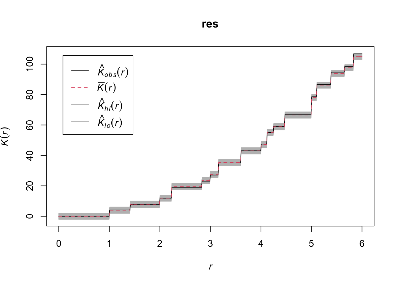
df <- read.table("./Grid2.txt", header = FALSE)

dim(df)
[1] 25 25coordinate <- function(database) {
# create blank vectors to store value
x <- rep(0, dim(database)[1] * dim(database)[2])
y <- rep(0, dim(database)[1] * dim(database)[2])
for (i in 1:dim(database)[1]) {
for (j in 1:dim(database)[2]) {
if (database[i, j] == 0) {
x[(i - 1) * dim(database)[2] + j] <- NA
y[(i - 1) * dim(database)[2] + j] <- NA
}
if (database[i, j] == 1) {
x[(i - 1) * dim(database)[2] + j] <- i
y[(i - 1) * dim(database)[2] + j] <- j
}
}
}
list(x = x, y = y)
}
mydata <- data.frame(x = coordinate(df)$x, y = coordinate(df)$y)
mydata <- mydata %>% filter(!is.na(x))
# visualize the grid
ggplot(mydata, aes(x = x, y = y)) +
geom_point() +
scale_x_continuous(breaks = seq(1, 25, 1)) +
scale_y_continuous(breaks = seq(1, 25, 1)) +
labs(title = "Grid 2")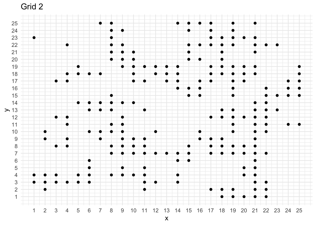
# number of points

print(paste("Number of points: ", mydata %>% nrow()))
[1] "Number of points: 221"n <- mydata %>% nrow()
library(spatstat)
# create window - a spatial ppp object
mydata_rr <- ppp(mydata$x, mydata$y, window = owin(c(1, 25), c(1, 25)))
# Creating multiple random point patterns with n points and within the window
set.seed(2020)
random_pattern_generator <- function(a) {
temp_v <- sample(c(0, 1), a * a, replace = T)
temp_df <- data.frame(matrix(temp_v, a, a))
simdata <- data.frame(x = coordinate(temp_df)$x, y = coordinate(temp_df)$y) %>% filter(!is.na(x))
simdata_rr <- ppp(simdata$x, simdata$y, window = owin(c(1, a), c(1, a)))
simdata_rr
}
ex <- expression(random_pattern_generator(25))
# Calculate the upper and lower boundaries
res <- envelope(mydata_rr, Kest, nsim = 99, simulate = ex, verbose = FALSE, saveall = TRUE, global = TRUE)
resSimultaneous critical envelopes for K(r)
and observed value for 'mydata_rr'
Edge correction: "iso"
Obtained from 99 evaluations of user-supplied expression
Envelope based on maximum deviation of K(r) from null value (estimated from a
separate set of 99 simulations)
Alternative: two.sided
Significance level of simultaneous Monte Carlo test: 1/100 = 0.01
............................................................
Math.label Description
r r distance argument r
obs hat(K)[obs](r) observed value of K(r) for data pattern
mmean bar(K)(r) sample mean of K(r) from simulations
lo hat(K)[lo](r) lower critical boundary for K(r)
hi hat(K)[hi](r) upper critical boundary for K(r)
............................................................
Default plot formula: .~r
where "." stands for 'obs', 'mmean', 'hi', 'lo'
Columns 'lo' and 'hi' will be plotted as shading (by default)
Recommended range of argument r: [0, 6]
Available range of argument r: [0, 6]plot(res)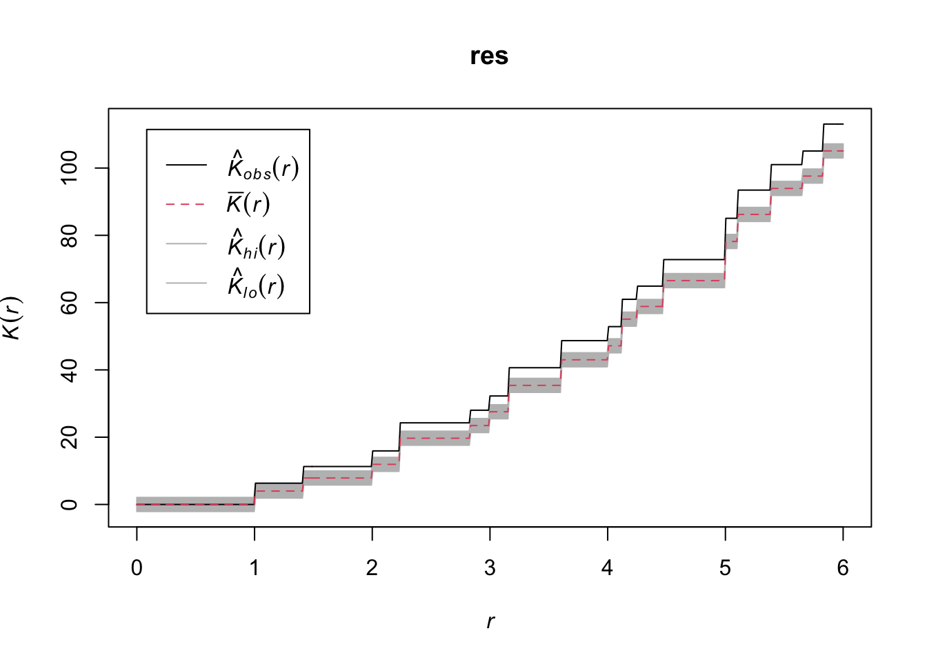
df <- read.table("./Grid3.txt", header = FALSE)

dim(df)
[1] 25 25coordinate <- function(database) {
# create blank vectors to store value
x <- rep(0, dim(database)[1] * dim(database)[2])
y <- rep(0, dim(database)[1] * dim(database)[2])
for (i in 1:dim(database)[1]) {
for (j in 1:dim(database)[2]) {
if (database[i, j] == 0) {
x[(i - 1) * dim(database)[2] + j] <- NA
y[(i - 1) * dim(database)[2] + j] <- NA
}
if (database[i, j] == 1) {
x[(i - 1) * dim(database)[2] + j] <- i
y[(i - 1) * dim(database)[2] + j] <- j
}
}
}
list(x = x, y = y)
}
mydata <- data.frame(x = coordinate(df)$x, y = coordinate(df)$y)
mydata <- mydata %>% filter(!is.na(x))
# visualize the grid
ggplot(mydata, aes(x = x, y = y)) +
geom_point() +
scale_x_continuous(breaks = seq(1, 25, 1)) +
scale_y_continuous(breaks = seq(1, 25, 1)) +
labs(title = "Grid 3")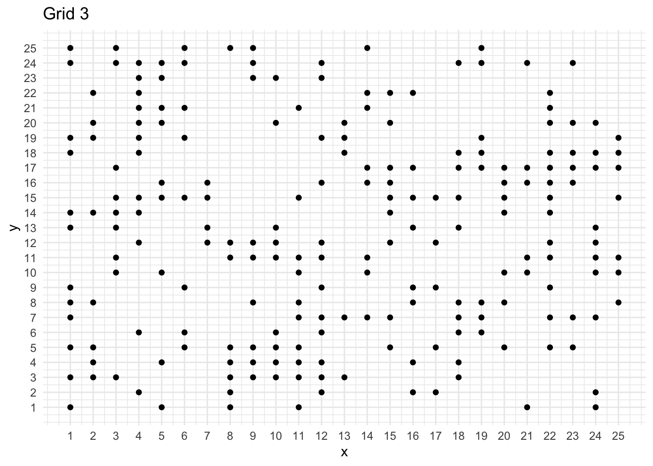
# number of points

print(paste("Number of points: ", mydata %>% nrow()))
[1] "Number of points: 213"n <- mydata %>% nrow()
library(spatstat)
# create window - a spatial ppp object
mydata_rr <- ppp(mydata$x, mydata$y, window = owin(c(1, 25), c(1, 25)))
# Creating multiple random point patterns with n points and within the window
set.seed(2020)
random_pattern_generator <- function(a) {
temp_v <- sample(c(0, 1), a * a, replace = T)
temp_df <- data.frame(matrix(temp_v, a, a))
simdata <- data.frame(x = coordinate(temp_df)$x, y = coordinate(temp_df)$y) %>% filter(!is.na(x))
simdata_rr <- ppp(simdata$x, simdata$y, window = owin(c(1, a), c(1, a)))
simdata_rr
}
ex <- expression(random_pattern_generator(25))
# Calculate the upper and lower boundaries
res <- envelope(mydata_rr, Kest, nsim = 99, simulate = ex, verbose = FALSE, saveall = TRUE, global = TRUE)
resSimultaneous critical envelopes for K(r)
and observed value for 'mydata_rr'
Edge correction: "iso"
Obtained from 99 evaluations of user-supplied expression
Envelope based on maximum deviation of K(r) from null value (estimated from a
separate set of 99 simulations)
Alternative: two.sided
Significance level of simultaneous Monte Carlo test: 1/100 = 0.01
............................................................
Math.label Description
r r distance argument r
obs hat(K)[obs](r) observed value of K(r) for data pattern
mmean bar(K)(r) sample mean of K(r) from simulations
lo hat(K)[lo](r) lower critical boundary for K(r)
hi hat(K)[hi](r) upper critical boundary for K(r)
............................................................
Default plot formula: .~r
where "." stands for 'obs', 'mmean', 'hi', 'lo'
Columns 'lo' and 'hi' will be plotted as shading (by default)
Recommended range of argument r: [0, 6]
Available range of argument r: [0, 6]plot(res)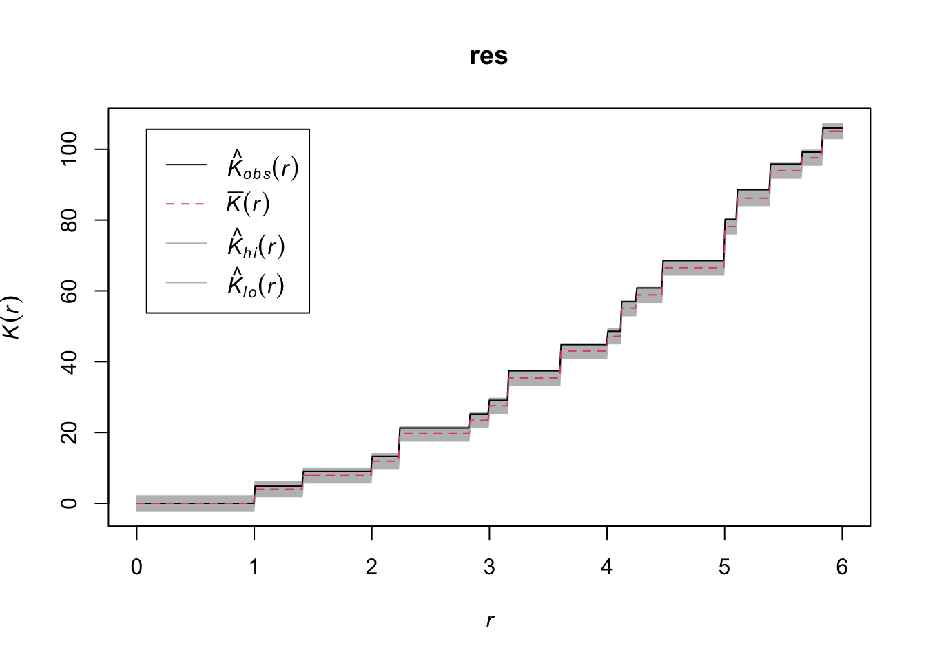
Reuse
Citation
@online{xu2020,
  author = {Keren Xu},
  editor = {},
  title = {Test {Random} {Pattern}},
  date = {2020-05-01},
  url = {https://xukeren.github.io//posts/2020-05-01-test-random-pattern},
  langid = {en}
}